This work has been done by Gilead Wurman with consultations
from Chris Crosby and Ramon Arrowsmith.We are working with the GRASS
GIS system to develop a 3D GIS and visualization system for our project.
GRASS link: http://grass.baylor.edu
Web log
In ancient times
The first few weeks working at this were spent coding a GIS from
scratch, under the assumption that no open-source GIS existed. Suffice
it to say this wasn't true, and the day I found out about GRASS I turned
to it as the basic foundation of the visualization project.
Visualizations using GRASS
The first real attempt at finding a visualization methodology
involved a 3D tool called NVIZ which is incorporated into GRASS. The
following images were generated using NVIZ from data stored in GRASS.
Download tiff
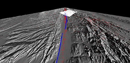
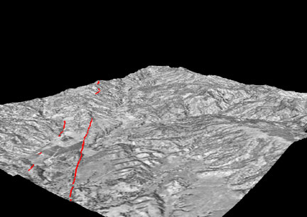
Shows an overlay of several features of NVIZ. The base 30m
DEM is hillshaded (this is done automatically by NVIZ with all elevation
data, and can be dynamically adjusted), and is set to 50% transparency
to allow hypocenter locations (red X's) to show underneath. These x's
are actually plotted volumetrically here, although they can be projected
to the elevation data if desired. The blue trace is the 1966 rupture
from Lienkaemper and Brown. Finally, the brighter patch is the Parkfield
DOQ overlaid on the 30m DEM. Note that this patch is not transparent,
and this was done using the DEM as a mask to delineate two different DEM
surfaces, one 50% transparent and one not. Vertical exaggeration here
is approximately 3x, and perspective is significantly exaggerated as well
(this is adjustable).
Download tiff
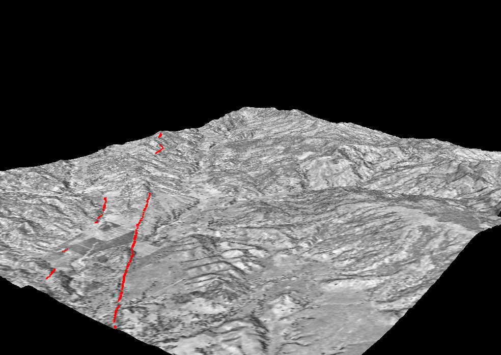
This is a closer in view of the Parkfield DOQ overlaid as a
color map on top of the 30m DEM, with the red trace showing the 66
rupture. Vertical exaggeration is still 3x or so.
Download tiff
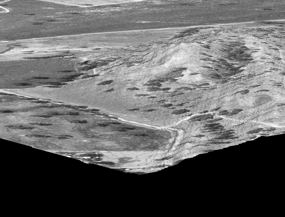
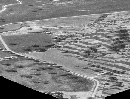
This and the next three images highlight a significant shortcoming
of both the NVIZ tool and GRASS in general, which we will have to address
in the coming months. This is a really close-in view of part of the
Parkfield DOQ overlaid on the 30m DEM. In this image, the polygon sampling
is 30m. The problem is that NVIZ can only assign each polygon one color,
meaning that the DOQ is severely undersampled and unintelligible when
you get close in.
Download tiff
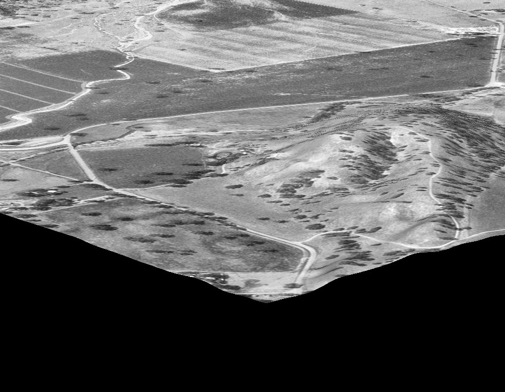
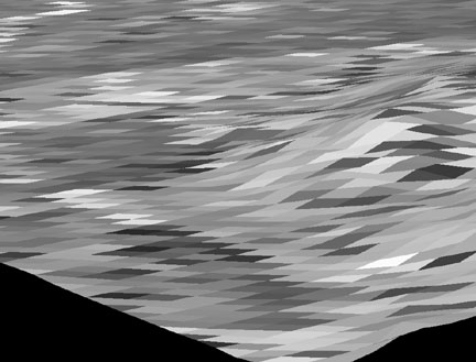
This is the same dataset sampled at 1m instead of 30m. Now we
see a different problem. The DOQ is quite detailed at this resolution,
and is very readable. The DEM, on the other hand, is now severely
OVERsampled, and as a result gets discretized and ugly. This is also
an unacceptable condition.

Download tiff
This is the best solution available now, which is to resample
the low resolution data set to the higher resolution. Obviously, this
is annoying as well as a sink for both RAM and disk space. In order
to resample this dataset I had to use a very simple interpolation (inverse-distance-weighted
average) and cut the dataset down to a region approximately 2.7km on
a side, so this can't even be done with the entire quad, let alone the
entire DEM. The results are obviously much better, with both the DEM
and the Quad looking reasonable, but the DEM still has a chunky look to
it, which would be solved by applying a spline interpolation instead of
the IDW average I used. Even with the dataset cut down to 2.7km square
and the less intensive IDW interpolation, resampling the DEM took about
an hour on cordillera (Sun Blade 2000). Obviously not ideal for our purposes.

Download tiff
Same as above, but with interpolation using regularized spline
with tension which took less processor time.
Commentary
- This highlights a general disadvantage of GRASS versus Arc,
which is that GRASS works with a project at only one resolution at
a time. So if you have multiple resolution datasets you have to make
tradeoffs in both visualization and analysis. I don't know that I have
the skills to recode this for the whole GRASS program (probably not),
but I may be able to trick the NVIZ tool into working around this somehow.
- It would be nice when we display the seismicity data to
be able to set the size or color of the data based on magnitude, uncertainty,
etc. These should be pretty easy to implement, so I'll work on that for
now.
- Another limitation is that NVIZ does not allow true 3D
positioning of the viewpoint, more like 2.5-D. You can position your
viewpoint anywhere in the XY plane, but your Z position can only be
positive right now, and even so when you go below the elevation of your
highest data point the scene flips over and goes wonky. That's a bit
more long-term. Also, the view target point can be set anywhere on the
elevation surface, but not above or below it. This is less limiting than
the viewpoint limitation, but I could see wanting to take level sets of
the data looking somewhere below the surface, for example.
- I have some good news to report about the resolution issues.
I found that GRASS has a "wish list message board" where you can post
your requests, so I posted one yesterday about the limitation that the
software can't display two different resolutions at once. Sure enough,
this morning one of the core programmers got back to me saying that a workaround
would be pretty simple for the 2-D display (not so much for NVIZ unfortunately,
but I'll take a look at that too).
Attempts with Vis5d+
In an attempt to improve upon the limited visualization capabilities
of NVIZ, I spent a day or two looking at a tool called Vis5d+, which
was designed to visualize results of atmospheric modeling. The
general conclusions are as follows, and also reiterated in the progress
report below.
- Vis5d+ is very specialized for atmospheric modeling, and
is hardcoded to read wind velocities
- While it is very good at visualizing volumes, it has limited
ability to display vector and 2D raster data, and no ability that I
can see to display point or site data
- It is even more one-resolution than GRASS. Not only
can it only display data in one resolution at once, but it is incapable
of reading irregularly spaced data in the first place, without additional
software (NetCDF).
- The data format is very much black-box. Files in
v5d format are binary and the specification is nonexistent as far as
I can tell. Conversion from other formats is through fortran/c
programs and is very fragile.
- As a side note, a conversion function exists between GRASS
and Vis5D data, which I never got to work properly, because Vis5D is
a deprecated older version of Vis5d+, and there is no backward compatibility.
2 April 2004
I played around with Vis5D a bit and have come to the following
conclusions. From a visualization standpoint it is worlds better
than NVIZ/GRASS. However, the data interface is simply craptastic.
Vis5D was designed as a vizualization tool for atmospheric model results,
so it is highly specialized in that direction. That is, it is hardcoded
to look for wind vectors using the variable names U,V,W in the data, etc.
Not that these couldn't be tricked into being GPS motion vectors or whatever,
but still, it's a bit of a hack.
Furthermore, Vis5D was really only designed to take regularly
gridded data, and is not very good at reading in and interpolating
irregular datasets. Right now there is an add-on module that allows
it to read irregular data in one particular format, NetCDF, which is
specialized for (you guessed it) atmospheric observations. With
a little bit of coding magic the same module can probably be made to
read in irregularly spaced geophysical data, but it will take time to
figure out exactly, since the data format is not at all transparent.
In the meantime, I have installed for myself the latest (non-release,
highly unstable) version of GRASS. This one promises to have
much better in-house 3D visualization capabilities, and in addition
to that I will look into interfacing GRASS data with Vis5D in some simpler-than-it-is-right-now
way.
And finally, we hit home
After some more flailing around, I talked to Marvin Simkin here at ASU, and found out
about a series of perl scripts he had written to make writing VRML
a little bit easier. With those scripts in hand, I began to work
on an interface between GRASS and Marvin's holodraw scripts, also in
perl.
Now our model for this project has solidified somewhat. GRASS
will be the database, since it is capable of georeferencing multiple
data sets effectively. A web form (to be designed by Jeff Conner)
will allow users to decide which data sets they want to query, in what
bounds, at what resolution, and how to display the results. The
web form will output an ASCII instruction file to my own perl scripts,
which will use those instructions to query GRASS and convert the data into
holodraw formatted ascii files. Marvin's scripts then convert the
holodraw file into a VRML file, and this file is posted on the web server
for download or online viewing by the user, using any VRML-capable browser
or plugin. This solves our rendering problem because the rendering
is done locally on the client side, and since VRML is a generic rendering
tool, it doesn't suffer from many of the limitations that NVIZ
and Vis5d+ have, since they are specialized to one degree or another.
In particular, VRML does not have any native resolution, which
will allow us to display multi-resolution datasets on top of one another.
14 May 2004
Unfortunately, I wasn't very productive on Thursday because
I spent a lot of time trying to hack together a way to read color scales
into the site data (to display points in different colors depending
on a random attribute), but after banging my head against it for a while
I decided in the final analysis to just leave it out altogether for the
pilot version.
I did write the corresponding code for the vector data today,
and I'm getting through the raster data right now. The latter
should be done by the end of next Thursday, when I come back in.
I am encountering some limitations on the way, however.
For starters, VRML 2 for some reason does not support line thickness,
so I can't give vector data width. Unfortunate, since VRML 1 has
the ability, but for some reason it wasn't included in 2. And
for the time being I
don't know if I can affect whether polygons are filled or not.
Also, I'm getting a bit scared of the file sizes coming out of
the raster datasets. The ascii GRD file representing the 30m DEM
is about 66 Mb by itself. This isn't so bad except that it may
be difficult to transmit to our users. We could probably zip it
up of course, that should give us a good 60% compression, since it is all
ascii, but we're still talking 20-30 Mb downloads, which for some people
could take a while. Just so's you're aware. We may want to put
a disclaimer on the webside.
Once I finish writing the raster code, I'll feel comfortable giving
Jeff an interface to work with, so hopefully we'll be underway on that
by next Friday. While he works on that end I'll continue working
on the ascii to vrml side of things. Looking at Marvin's code,
it is optimized for GMT, which is unfortunately much smarter than GRASS
in certain respects. I have been making an effort to output GMT-style
ascii files out of my scripts, but I suspect I will need to rework some
of Marvin's codes to get things running smoothly. I'll keep you
posted of course.
21 May 2004
The first proof-of-concept VRML files are done!
This VRML file shows off a couple of features that have been
implemented. The red line is the surface trace of the 1966 rupture
after Lienkaemper and Brown, which has been projected to the surface
of the 30m DEM (not shown), so it's actually in 3D. The spheres
represent seismicity in that area from the NCSN catalog (from July 1966
to Feb 2004). The radius of each sphere is (Mag*100 + 10) meters,
and the color is roughly the age of the event from cyan (old) to magenta
(recent). It's not actually the age of the event since I haven't
figured out a good way to convert date/time to a usable value for color,
but I used index as a proxy since the list is in chronological order. The
bounding box was added easily using one of Marvin's scripts, and scales itself
automatically to any VRML scene it is applied to. There are customization
options for tick spacing, dimensions, etc., but for the time being I think
we'll leave it on automatic rather than worry about yet another set of
forms and scripts. The region is about 2km on a side, and about 18km
deep. I haven't yet implemented 3D regions in the query commands,
so while I can limit the horizontal extent of the query, the vertical extent
is going to be whatever the vertical extent of the data is.
Next on the chopping block, there are a couple of scripts that
need to be written out (one to make the color palettes, for example, I
made this one by hand), and some serious code documentation needs to happen.
Finally, the script for rasters and DEMs needs to be done. The
non-DEM rasters might be easy enough, but to make the DEMs in VRML I
need to add to Marvin's code, since he didn't implement the ElevationGrid
VRML geometry yet. Further along we'll look at the other big thing
we were missing, draping rasters on elevation grids. Should be possible
as long as we trick VRML into thinking the raster is a texturemap, and
maybe pad it to make it the right size.
Which brings me to the one serious limitation of VRML: it doesn't
know what "null" means. Instead of saying "there is no data in
this part of the grid" I have to pad the DEM or raster with zeroes, which
is not really optimal. But so far, that's the only thing I've run
into.
28 May 2004
This week I figured out how to make ElevationGrid geometry
useful to our application. This involves a bit of hackery, for several
reasons. First, the ElevationGrid geometry is hardcoded in VRML
to represent elevation change in the y-direction on an x-z plane. Since
our elevation direction is z, this requires rotating the whole grid 90
degrees around the y-axis. Also, holodraw does not yet implement
ElevationGrid. I talked to Marvin about this and he will work on
it over the next few weeks. I tried copying his scripting to implement
it myself, but I got lazy pretty quickly, hence the next major hack.
Rather than writing my perl script to create holodraw directives,
I wrote this one to write VRML itself. It's a bit more awkward
than using holodraw, but it's much easier for me than interpreting someone
else's code :-)
Anyway, the new demo area with the DEM on top is here.
There are a couple of things that bear addressing soon.
- The zero-width line used to depict the fault is no longer
adequate. Because of (presumably) aliasing issues, the vector
does not map exactly to the DEM as intended. Instead, it weaves
in and out of it, so in effect part of the fault trace is over the surface
and part is underneath. I have tried a couple of different tricks
to get the line to show up properly. First, I used holodraw "polygon"
directives to make the line into vertical panels of some height. This
is a little better, as part of the panel is almost always poking above
and below the terrain at once, but I want to make the line emissive rather
than reflective, and holdraw doesn't support that (native VRML does). I
also tried making the line an extrusion of a circle (well, an octagon).
The results of this are more promising, as the fault looks great
by
itself, but there is some kind of clipping issue going on when I
put it on the
DEM, which I will try to address at some later time.
- The bounding box does not encompass the DEM (nor my extrusion-type
fault trace) automatically, which is to be expected. All this means
is that I have to implement the user-defined bounding box options in
my scripts, which should take very little time.
- In the slightly longer term, colormapping needs to be worked
out, and I'm not sure how that happens with ElevationGrid (though I'm
fairly sure it does somehow).
Also, the flat raster has not been implemented yet (shouldn't
be a big deal, just a series of polygons), and there are a couple of
small holes that need to be patched up in other scripts.
Finally, all the little scripts that were waiting to be written
have been (more or less), and code has been documented (more or less).
Next week I'm getting together with Jeff on Tuesday to chew on
the web side of things.
1 June 2004
Short week, I only worked tuesday. Jeff and I spent some
time installing grass5.3 as root (I had it installed locally for myself
previously) and we have installed PostgreSQL. This confirms that
permissions can be appropriately set to allow outside users to access the
database in GRASS.
Also, I implemented color scaling of the DEM, and the results are
available here.
I set up two directional lights from the SW at 45 degrees from
above and below, to illuminate both the top and underside of the DEM
(otherwise the DEM was hard to see from below. I either need to
reconcile the use of directional lighting on the DEM with headlighting
on the seismicity spheres, or I need to learn to live with the fact that
the user will have to keep switching their headlight on and off. I
find the latter more likely :-)
Also, I fixed up the vector representation a bit, by a) making
the color emissive rather than diffuse, b) making the solid variable
false, so both sides of each polygon get rendered, and c) realizing
that I was defining my cross-section inside out (i.e., clockwise instead
of counter-clockwise) so I set the ccw variable to false. Still
not perfect, but good enough for now. I am considering trying the
vertical plane implementation again with emissive color. We'll
see.
Finally, I implemented all the options for tick formatting and
manual setting of bounds for the bounding box.
Next tuesday Jeff and I will get together again to get the PostgreSQL
database hooked into GRASS, and in the meantime he will be writing the
front end of the web form.
8 June 2004
No progress this week on the database due to a hardware emergency
that Jeff had to address. However, I used the time to work out
a way to drape images over a DEM. I am happy to say that the whole
resolution issue that we saw with NVIZ is absent. The results are
here.
Incidentally, this is also probably the easiest way to create level
rasters, and I'll work on that next week.
Some issues:
- The color palettes available for texturemapping are those
internal to GRASS, which are different from the GMT palettes I used for
everything else. This inconsistency is mildly annoying but not
critical.
- The texture image has to be the exact same dimensions as the
surface it is being mapped to, otherwise it will just get distorted to
the same shape. Right now also not so much of an issue because I
have it hardcoded to pull an image with the exact same dimensions as the
DEM.
- Slightly more serious, I think there is a slight mismatch
between the DEM and everything else right now, owing to the fact that
GRASS outputs one elevation point for each grid square, and VRML wants
one for each vertex. I'll work on a solution to this next week,
it will probably involve padding the region with one more grid point on
the S and E sides for the one operation, and then offsetting the whole
business by half a grid square in each direction.
That's about it. I tried the vertical plane implementation
for vectors again, and decided once again that I prefer the tube implementation,
so we're sticking with that.
16 June 2004
Jeff and I got together today to link the PostgreSQL database
to GRASS and decided collectively that the interface is obtuse and useless.
Instead, we are going to try to query GRASS as needed by examining
the filesystem. While it's not as convenient as using the Postgres
JavaScript commands, it seems like less pain than actually synching the
Postgres database with GRASS.
We also got our heads together and came up with a semi-solid design
for the web form, including how we would populate the various list boxes
for rasters, sites, etc. Jeff will work on that over the next few
days, and that should be done by the end of next week.
On the other end of things, I am bit by bit adding functionality
to the perl scripts. The focus of this week was separating out the
displaying of flat rasters from DEMs and rasters draped on DEMs. Initially
this was all lumped together in one script, but after examining the requirements
for each function I decided there was almost no overlap and they should
be separated out. So, now they are.
Finally, I'm beginning to turn my eyes toward addressing 3D datasets.
More on this next week, but right now I'm still fighting with the
little quirks of GRASS with regards to 3D. GRASS does generate something
called a display file or dspf, which in principle should be a list of polygons
in an isosurface, but based on my prior experience with GRASS, they will
not be in any kind of readable or exportable format.
1 July 2004
Been a couple of weeks, not a whole lot of progress on the scripts
themselves. Good news is much progress has been made on the web front-end,
and the whole thing should be ready to go within a week or two.
The one thing that has been done script-side is to make the vectors
look nicer by interpolating the elevation between the three nearest points
when mapping the vector to a surface. Previously the value of the
nearest point was taken, and that caused the vector to spike above the
terrain or plunge below it. Now the vector follows the terrain exactly,
at the minor cost that it takes about 3 times as long to generate the VRML.
Since this isn't speed-sensitive it's not a big deal. The rendering
in the browser takes the same amount of time. Compare the results
between the last rendition
and this most recent
one.
In other news, I've decided to put off the 3D stuff until after the
demo version is out. It's just too big a pain in the butt right
now, and maybe after the demo we'll get some nicer datasets and maybe
even some advice from potential users (or help?). I know Marvin
has rendered isosurfaces in VRML so I'll probably talk to him sometime
soon.
16 July 2004
The last couple of weeks have been spent making the JSP web form
work harmoniously with the scripts I have written (not as easy as it may
sound). There are a couple of final touches and functionality that
needs to be added, and the we will be ready to put it up for the world
to see.
On the script end a few moderate changes have been made. I am
now using a revised version of holodraw which allows me to embed VRML directly
into the holodraw file rather than as a separate .wrl file. So now
instead of mucking around with catting several different files in the right
order, it all goes into the draw file and gets sorted out there. So
that's much cleaner.
I also added some scripting at the end to take all the results and
move them off into a unique directory. This will avoid the problem
of different requests potentially overwriting each other's data. The
script also packages all the relevant files into a .tar.gz for easy download
by the user.
Finally I added a couple of checks to stop up the gaping security holes
I've left in the code, so while we may still be vulnerable somewhere (you'll
get no guarantees from me) it won't be easy enough for a two-year-old to
do it.
21 July 2004
The web form now has a button to initiate the scripts and the output
is placed in a web-accessible directory on cordillera. So basically
this means the tool is ready to debut. There are a couple of other
elements we would like to add before posting it online, mostly dealing with
notifying the user at various stages of the process. The sites form
hasn't been implemented yet, but we can post with that part labeled "under
construction" and add it on later.
12 August 2004
Finally! We have a working version of the web form after many
hangups. We still have a few sticking points to sort out, but the form
can be accessed at http://agassiz.la.asu.edu:8080/gservlet
(changed 12-Oct-04). Here are some example values to enter that should
give you some nice looking output:
enter a region with
North=3983700 South=3981012 West=724948 East=726320
press add_region
Enter 2 Vectors:
Vector1:
Vector File=Rupture66 Height=(surface)DEM_30m thickness=5 color=255,0,0
press add_vector
Vector2:
Vector File=Landslides Height=(surface)DEM_30m thickness=5 color=0,0,255
press add_vector
Enter an elevation:
Raster File=DEM_30m Options=(texture)Parkfield_Quad
press add_elevation
Enter a bounding box:
color=255,255,255
bounds=(manual) north=3983700 south=3981012 east=726320 west=724948
top=1000 bottom=0
ticks=auto
press add_bounding_box
Press Finish
Fill out an e-mail address. This part isn't working yet but Jeff will
be working on it this week to hopefully resolve the issues we are having
with it. When it is working it sends an e-mail to the address entered
when the server has finished processing the request. When you have
finished entering an e-mail address press start. The server will process
the request and upon completion present the user with another page with
a link to the wrl page.
Suggestions for improvements will have to wait until I figure out a way
to receive them without flooding my email. I am looking into setting
up a discussion forum for this purpose. In the meantime, we will be
accepting additional geophysical data for the Parkfield area database. If
you have data for this region please email gwurman@asu.edu with a link to
the data (please do not email the data as an attachment if it is more than
a few KB in size). The extent of the study area is currently (meters
northing and easting, UTM zone 10N, NAD83 datum):
north: 4001536
south: 3915882
west: 706744
east: 772417
Any data within these bounds (or slightly out of these bounds) is welcome
27 August 2004
The webform is nearing release readiness. All that is left is
to implement the sites-query portion of the form, which is a bit complicated
as it requires updating column headers on the fly as the user selects different
sites files to display. Once this is complete, we will email out the
location to people so we can get some reactions.
Meanwhile, I have been working on expanding the DOQ coverage in our dataset.
Previously only the Parkfield USGS quad had been covered, but now the
coverage is a 4x4 patch from Smith Mountain (NW) to Orchard Peak (SE), which
is called simply "Orthophoto" in the database. Someday we will expand
this coverage, and probably add 10m DEM coverage over the study area. Someday.
While this was going on we discovered that our disk space on cordillera
was exhausted, so we took the opportunity to port the whole business over
to the GEON data node. Now we have a nice big (just under 2 Tb) playground.
Bring on the data! Also, this is the final logistical arrangement,
so no more moving files and recompiling code in new locations. Yeehaw.
12 October 2004
The last month plus has been spent correcting minor bugs and adding some
last-minute functionality to the system. In addition, in case you missed
the huge link at the top of this page, I've taken data from the recent Parkfield
earthquake and visualized it using the PUVP system. Well, actually I
did a bit by hand in VRML, because this visualization showcases functionality
that will eventually be in the system but hasn't been written yet. Check
it out here.
We are currently in alpha testing within the group prior to widespread release
of the website. Before we do this we also are looking into establishing
a forum somewhere to accommodate the interactions that will take place when
it is released, including bug reports, improvement suggestions, code requests,
etc. Once this is done I think we will release the page. In the
meantime, the link is http://agassiz.la.asu.edu:8080/gservlet.
Some notes about the web page, if you are interested in toying with
it:
At present, the user interface is not very streamlined and not too user-friendly.
To help you get started, we have provided the following aids:
-There are some demo scenes that can be generated using buttons at the top
of the form. This should help you get a feel for the capabilities of
the software.
-Among the links at the top of the page is a tutorial which will guide you
step-by-step in creating the demo scenes by hand.
-Another link leads to a detailed documentation page with guidance on each
function on the page. If you wish to create your own queries, it is
*highly* recommended that you do so with this documentation page open as a
handy reference.
-Yet another link leads to a PDF overview map of the study area. This
should help you zero in on the area you are interested in, and also shows
the boundaries of some of the datasets.
There are a couple of currently known issues that will need to be worked
out eventually:
-The system has only been tested under MS Internet Explorer in Windows.
We know for a fact that it doesn't work with Netscape in Windows. The
lack of a freeware VRML client for UNIX/Linux has prevented testing in
those operating systems.
-On the final page before submitting processing, the program asks for an
email to notify you when the job is done. If "return" is typed rather
than clicking on the "Start" button, this leads to a server error. Press
the back button and click Start.
Completed as part of NSF grant EAR-0310357 "Kilometer-scale fault zone
structure and Kinematics along the San Andreas Fault near Parkfield,
California" supervised by Dr. Ramon Arrowsmith at Arizona State University,
Tempe, AZ.
Page maintained by Gilead Wurman and Prof. Ramón Arrowsmith
Last modified May 21, 2004