This document will describe the basic operation and application of the Leica Total Station surveying equipment as well as discuss the process of downloading the data and producing detailed topography maps using the Liscad software. It is meant to explain the operation based upon the Active Tectonics members’ experiences in using the equipment, and should supplement the reading of the manual and your intuition. This document contains the basic set-up and operating instructions for our electronic surveying equipment. It also contains discussions of how the instrument works, and suggestions for methods and strategies of use.

Most of this equipment is stored in the locked cabinet, or alongside it, in the Active Tectonics lab, room 475 of the Physical Sciences H-wing. An equipment list and check out sheet are posted on the door of the cabinet.

The Leica (Wild) equipment is well known as some of the best surveying equipment available. It is often referred to as "the Cadillac" of surveying equipment. "All surveyors either own a Leica (Wild) or wish that they did" (Hanz Haselbach, Jr., personal communication, 1991). Leica (Wild) makes top of the line equipment that is used on all expeditions and has better mechanics, optics, factory support, ease of repair, and ability to maintain resale value than other manufacturers. Furthermore, the company supports older equipment by providing a modular set-up, allowing selective upgrades:

In order to properly prepare for a survey effort, checking the equipment in the lab/office before leaving and proper reconnaissance before set up are important. On the next page is a list of equipment and the checks that should be made before leaving the office.

Before leaving the office, look at the base map or airphoto of the area and define the mapping project(s). Consider access. If you need permission to get on the property, you should get that well in advance. The equipment is heavy and bulky. Two people can carry it with difficulty for 1 or 2 kilometers, but it is a demoralizing experience. Therefore, try to plan appropriate vehicle access, but don't drive unnecessarily through the landscape destroying the beauty and making a bad name for geologists! You must have a field assistant. Operating this equipment by yourself is pretty silly, although it can be done. You will end up walking at least two times the total slope length of the shots you make. The distance will add up quickly! Your helper need not be a geologist, but should be sturdy, careful, and interested.

Once in the field, walk over the area with the field assistant. Look for suitable instrument stations. Much time and precision may be lost with multiple set ups. Therefore, plan the minimum number of instrument stations. A high position somewhere near the survey area should suffice. Remember that the instrument has an effective working range of at least 1 km, so if you have walkie-talkies or body signals and can communicate (see communication techniques) over long ranges, much of the survey may be completed from a single well chosen site. Consider gullies and ridges, and other obstacles that may obscure the survey. Remember that the reflector plumb staff telescopes to 2.15 m, so that may help with visibility. Be sure to communicate to the instrument operator changes in reflector height (click here to see how to enter into Total Station) and record them on the Survey Record Form and in the Thoedolite! While reconnoitering the area, consider the problem being addressed by the mapping project, and choose an appropriate and optimal strategy: What is the optimum number and distribution of points necessary for this project? What is the desired precision? Will I ever want to reoccupy this network? Be sure that the field assistant understands the strategy too, so that you do not have to have major discussions about strategy once you have started working, although the plan should be flexible if an obvious modification becomes apparent.

Choose an adequate instrument station as described above. In detail, ensure that you can safely operate the instrument without knocking it over. It is necessary to have the center of the instrument, which is the point of intersection of the transverse axis and the vertical axis of the instrument, directly over a given point on the ground (the Instrument Station). Also, the circle and the transverse axis must be horizontal (Moffitt, 1987). Remove the yellow plastic cap from the tripod, and leave the instrument in the case until the tripod is nearly level (see below). The tripod legs are spread (not too vertical) and their points are placed so that the tripod is approximately horizontal and the telescope is at a convenient height for sighting (this is important: you don't want to get a sore back from it being too low, nor do you want to get sore calves and fall over from it being too high). The instrument should be within 20 cm of the desired point, but no extra care is taken to set it up closely at once. If the location of the instrument station is not predetermined, set up first, and then use the optical plummet to locate the benchmark: this will save time, because it takes extra care to accurately set up over a benchmark. When setting up on rough ground, two legs of the tripod should be set at about the same elevation and the top of the tripod is made level by changing the length of the third. Consider the common sighting direction and try to have one leg pointing that way so that there will be a gap between two legs behind, and the instrument operator will not have to straddle a tripod leg for the entire session. If the instrument is more than a few inches from the given point, the tripod is shifted bodily without changing the inclination of the legs and it is set near as possible to the point. Check the level by placing a Brunton compass on top of the tripod and adjusting gently until the Brunton bubble level indicates that the top of the tripod is level. Tread tripod shoes firmly into the ground, making sure to press along the leg and not verically down (Anderson and Mikhail, 1989). If shoes do not penetrate to an equal depth, re-level by extending or retracting the tripod legs. Before attaching the instrument, check that the clamps of the telescopic legs are tight.

Once the tripod is nearly level and nearly above the desired point, remove the Theodolite gently from its case and carry it with one hand on the upper handle, and one hand below, to the top of the tripod, and immediately screw the tripod fixing screw firmly into the bottom of the theodolite. The levels on the instrument are very sensitive, and therefore, the instrument should be completely set up in order to ensure that it will be properly leveled. This will also give the tripod more time to thermally equilibrate with the atmosphere and incident sunlight, since differential thermal expansion of the tripod legs will effect the levels.

Now you are ready for fine leveling of the instrument. Use the three black footscrews on the tribrach (the device on the bottom of the Theodolite to which the tripod fixing screw is attached) to center the circular bubble. This is a coarse level. Turn the outer ring on the eyepiece of the optical plummet until the crosshairs are in focus. Turn the inner ring of the optical plummet until the ground point is in focus. Slacken tripod fixing screw and move instrument over tripod plate until cross hairs coincide with ground mark. Only translate the instrument over the tripod plate, do not rotate it. Finally retighten fixing screw. Now do the fine leveling.

Note that the instrument will drift out of level as the day progresses. Repeat the above steps as needed and enter change by pressing the level button (see Operation). If the optical plummet is not above the ground point desired, slacken tripod fixing screw and move instrument over tripod plate until cross hairs coincide with ground mark. Only translate the instrument over the tripod plate, do not rotate. Retighten fixing screw. Now press the ON button and the startup menu will come on. 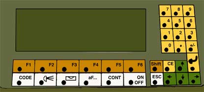Press the white LEVEL (figure 1) key along the bottom of the key panel followed by continue. When the levels are set press the continue button.

Now that the instrument is leveled up, set up and test the electronics. First, insert the Verbatim SRAM card into the slot in the Theodolite. Ensure that the arrow on the back of the card faces down when you insert it. See below for a suggested initial key sequence for the Theodolite and see the TPS-System 1000 Short Instructions System manual in the Theodolite case for a list of commands for the Theodolite. The keypad on the Theodolite allows for maximum utility with the minimum number of keys. Therefore, most of the keys have several functions, depending upon the class of operation. One way to remember the meaning is by noting the background color of the keys.

The ENTER button is important in that it executes the preceding commands or answers in the affirmative, while the CE button often clears the last command. Before anything, start with a fresh copy of the Survey Record Form, and fill out the important details at the top. Use this form to take notes while surveying. Remember to record all observations and considerations, since the next time you look at this data, it might 6 months from now in the Dungeon! Record the observations so that someone else can understand. After all, someone else might use the data.

Now that the instrument has been set up physically and electronically, you are ready for operations.

Check to make sure that the reflector is properly mounted on the plumb pole by squeezing the small button on the lower back portion of the reflector as you slip it down over the top of the plumb pole. When you point the telescope at the reflector, the cross hairs must intersect on the yellow reflector plate as shown in Figure 1. This offset from the actual reflector is the same as the offset between the center of the telescope and the EDM.

We also have a Triple Tilt Prism Assembly that is used for longer distances .

Focus the reticle cross hairs by pointing the telescope at some other uniformly light surface (the sky), and rotate the inner black portion of the eyepiece until the cross hairs are sharp and black.

Point telescope toward reflector by means of optical sight. Use of this sight will speed up acquisition of the reflector significantly. With both eyes open, have the image of the white cross hair in the optical sight in one eye, and the reflector in the other. When the two are superimposed, you are approximately on target. This saves a significant amount of time searching for the reflector with the actual telescope.

The horizontal and vertical rotations of the Theodolite are controlled in two ways. First you can rotate the Theodolite horizontally by hand by placing two hands on either side of it and rotating it. To rotate vertically, rotate the EDM unit up or down by hand by nudging in up or down. Manual rotation works best and is less demanding on the battery if there is a distance change from point to point of several meters. Otherwise fine-tuning is done by turning the horizontal and vertical knobs on the sides of the unit.

The instrument updates angle measurements within 0.3 seconds, so the angles can be quickly displayed. In order to see the horizontal and vertical angles of the current pointing, push F2 (DIST). Before the station is moved press F3 (REC) to record the point.

As you are surveying it may be advantageous to switch operators occasionally. Another important hint is to have simple hand signals to communicate the status of the measurement to the reflector person or the type of topography to the instrument person without having to shout or use the two-way radios for simple communications (See Communication techniques). I like to have the instrument person hold his or her arm straight up when starting to focus and measure to indicate to the reflector person that he or she should hold the reflector level. As soon as the distance measurement appears in the LCD, the instrument person's arm is held sideways to indicate that the shot is complete and the reflector person should move to the next target point. With this scheme, approximately 100 points per hour can be acquired. Our record for one day is 707 shots with three people rotating through the two positions. If the target points are further apart or in rough terrain, you may have two reflector people, and alternate shots between them. This will speed up operations, but it requires more coordination and concentration, especially on the part of the instrument person.

Your surveying team may not be blessed with radio communication. However, there are some basic arm signals that we have developed for geomorphic features.

	"Shoot topo points."		"I'm ready to shoot point, please level the staff."
	"End that series."
	"That was the first point for a linear feature (fault)."
	"That was the first point for a breakline."

Coding specific points and breaklines

Lastly, save excel worksheet with a .ex extension. This file will be the master archive for your data. From it you can manipulate, plot, and contour your data. Print this file out and save the hardcopy somewhere safe.

Care

Hz. The length of one cycle is called the wavelength (l), which can be determined as a function of the frequency from

The speed of electromagnetic waves in a vacuum is called the speed of light, c, and is taken to be 299,792,458 m s-1.(Price, 1989). The accuracy of an EDM instrument depends ultimately on the accuracy of the estimated velocity of the electromagnetic wave through the atmosphere (Burnside, 1991).

where Amax is the maximum amplitude developed by the source, A0 is the reference amplitude, and f is the phase angle which completes a cycle in 2¹ radians or 360°.

The distance from instrument to reflector is D, l_m is the wavelength of the measuring unit, n is the integer number of wavelengths traveled by the wave, and Dl_m is the fraction of the wavelength traveled by the wave. Therefore, the distance D is made of two separate elements. An EDM instrument using continuous electromagnetic waves can only determine Dl_m by phase comparison (Figure 4).

If the phase angle of the transmitted wave measured at the instrument is f₁, and the phase angle measured on receipt is f₂, then

The phase angle f₂ can apply to any incoming wavelength, so phase comparison will only provide a determination of the fraction of a wavelength traveled by the wave, leaving the total number, n, ambiguous (Price, 1989).

Figure 4. Phase comparison. (a) An EDM is set up at A and a reflector at B for determination of the slope length (D). During measurement, an electromagnetic wave is continuously transmitted from A towards B where it is reflected back to A. (b) The electromagnetic wave path from A to B has been shown, and for clarity, the same sequence is shown in (c), but the return wave has ben opened out. Points A and A' are effectively the same, since the transmitter and receiver would eb side by side in the same unit at A. The lowermost portion also isslustrates the ideal of modulation of the carrier wave by the measuring wave. From Price and Uren, 1989.

For many EDM instruments, an accuracy in measurement between 1 and 10 mm is specified at short ranges, and a phase resolution of 1 in 10,000 is normal. Assuming an accuracy of at least 1 mm, therefore, a measuring wavelength (l_m) of 10 m is required. Approximating the speed of propagation, v, by 3 x 10⁸ m s^-1, 10 m corresponds to a frequency of 30 MHz. Adequate propagation of an electromagnetic signal of 30 MHz frequency for EDM purposes is not practical, so a higher frequency carrier wave is used and modulated by the measuring wave (Figure 5, (Price, 1989)). In the case of our instrument, the carrier wave is infra-red, with a wavelength of 0.835 µm, corresponding to a frequency of 3.6 x 10⁵ GHz.

The return signal is usually amplified, and then the phase difference is determined digitally. The signal derived from the modulation triggers off the counting mechanism every time the signal changes from negative to positive. The signal derived from the reflected ray stops the counting mechanism (Burnside, 1991). For our instrument, the integer ambiguity (n) of wavelengths is determined using the coarse measurement frequency of 74,927 Hz, equivalent to 2000 m, and the amplitude modulation of 4,870,255 Hz (30.7692 m) provides the fine measurement (Dl_m). In order to achieve the stated accuracy of 5 mm, the phase measurements are accurate to 1 part in 6,154.

where: DD₁ = atmospheric correction (ppm), p = atmospheric pressure (mb), and t = ambient temperature (°C). For extreme conditions of 30°C temperature change and 100 mb pressure change, one can expect variations in scale error of 50 ppm in a day. This maximum value is ten times greater than the stated initial accuracy of the instrument, and therefore should be accounted for by adjusting the scale error on the theodolite occasionally during the day's surveying effort (see Figure 6, graph 1 to determine DD₁).

where DD₂ = reduction to MSL in ppm, H = height of EDM above MSL, and R = 6378 km (earth radius). This correction is a constant and should be determined at the beginning of the survey effort by consulting Figure 6, graph 2a or 2b.

where D is the corrected slope distance in mm, D₀ is the measured (uncorrected) slope distance in mm, (deltaD) = sum of scale corrections (n is the number of scale corrections) in ppm, and mm = prism constant in mm.

The theodolite computes horizontal distance (D_h) and height difference (e_h) by accounting for earth curvature and mean refractive index. These corrections are on the order of 10^-8 or 0.01 ppm of D₀ and therefore not significant compared to the scale correction (~50 to 100 ppm).

Figure 6. Scale correction graphs from Theodolite manual. Use these to determine DD (sum of scale corrections).

Infra-red radiation from a GaAs lasing diode

The source of the IR radiation for our instrument is a Gallium Arsenide (GaAs) lasing diode. This device is made from a small chip of semiconducting material, and is similar in size and appearance to other semiconducting devices (Figure 7). Driven by a forward biased voltage and maintained by different electrostatic potentials in the two halves of the diode, an electron population inversion between the two halves of the diode will provide the energy level transition for stimulated emission of photons by electrons as they fall to the lower energy state (Price, 1989). The energy difference is emitted as radiation (and thus the process and device are called a laser--Light Amplification by the Stimulated Emission of Radiation). The process of stimulated emission enables the laser to emit an intense, monochromatic radiation that travels as a narrow beam for considerable distances before it spreads out (Price, 1989). The intensity of the IR radiation is nearly linearly proportional to the current flow and with virtually an instantaneous response (Burnside, 1991). If an alternating voltage is superimposed upon the normal operating voltage of the GaAs diode, the intensity of its emitted radiation varies in sympathy with the alternating voltage (Figure 8, Price, 1989). This provides a simple and inexpensive means of directly modulating the infra-red beam.

The GaAs diode is widely used in surveying. The small dimensions of the junction in which the radiation is emitted gives rise to poorer collimation of the radiation. Therefore, the GaAs laser emits a beam with a relatively large elliptical spread and the brightness of the GaAs laser is lower than that of other lasers. The spectral width of the radiation emitted is usually 2-3 nm compared with 0.001 nm of the visible light, HeNe gas laser and thus the GaAs laser lacks the monochromacity of other lasers, contributing error to the effective propagation velocity. However, GaAs lasers can be made to operate at orders of magnitude greater efficiency than other lasers, can be made much smaller and more rugged, and are considerably less expensive than other lasers (Price, 1989).

Because of the relatively low power radiated, a beam of sufficient power will not be reflected from an unprepared surface. A special reflector is therefore used in order to ensure a good return signal. A plane mirror can be employed, but it requires accurate setting, so in practice, a corner cube reflector is most often used. This reflector will return a beam along a path parallel to the incident path over a wide range of angles of incidence onto the front surface. A cube of glass is usually used with its edges ground into a corner with accuracies of grinding to within a few degrees of arc (Burnside, 1991). The path length of the signal within the reflector must be corrected for, and that is the reason for the setting of the prism constant within the theodolite. The constant for Wild circular prisms is 0. Note that over short distances, the "cat-eye" type reflector commonly used for bicycles will adequately reflect highly oblique incident signals.

Figure 7. Gallium arsenide diode characteristics. From Burnside, 1991.


Figure 8. Modulation of a Gallium arsenide diode. From Price and Uren, 1989.

Selected Technical Data--Leica (Wild) DI4L

The point over which the Total Station is set up is called an instrument station. Such a point should be marked as accurately as possibly on some firm object. On many surveys, each station is marked by a wooden stake, spike, or piece of REBAR driven flush with the ground and into the top of which a small (~ mm diameter) dimple is marked (a tack may be put in the wooden stake) (Moffitt, 1987). The Total Station measurements and reductions are made relative to the instrument station (E₀, N₀, and H₀--where E refers to distance East, N distance North, and H elevation, and the subscript ₀ indicates a reference value). These values must be predetermined by other means (triangulation, previous survey location, Global Positioning System, etc., or they may be arbitrary). In fact, for most local surveys, with only one survey set up, the instrument station is commonly taken to be (0, 0, 0).

In the lower portion of Figure 9, the geometric reductions in a vertical plane are indicated. From the fundamental measurements and a few more observations, the horizontal distance (HD) and elevation (H) may be determined:

(9)

H^* is the elevation difference between instrument and reflector, IH is instrument Height, and PH is the Prism Height.

(10)

Figure 9. Surveying geometry.

Determinations in the horizontal plane

In the upper portion of Figure 9, the map view reductions from the fundamental measurements are shown. Because we are interested in the map relations of the surveyed objects or observations, the distances East (E) and North (N) may be determined in the following way:

(11)

(12)

Foresight and Backsight: the traverse

One other thing that people have trouble with and that I have only recently gotten to the bottom of is the traverse or how you move your station to a new position. The figure below shows how one starts of at the reference position E0, N0, H0, works, and then moves to the new station with a reference position E1, N1, H1. What you have to do is shoot from the first location to the second (foresight) and record the E1, N1, H1, and the bearing Hz0. Then, move to the new location, set up, tell the total station you are at E1, N1, H1, and set the horizontal circle to Hz1 or Hz0+180 degrees (backsight). Then shoot to the reflector set up at the first station and record the position. It should be within a few mm of the original E0, N0, H0.

Precision

The angular accuracy at one standard deviation of the Theodolite is 3", and the linear accuracy at one standard deviation of the EDM is 5 mm ± 5 ppm of the slope length. The upper portion of Figure 10 shows a map view of the 1 standard deviation error volume (remember that the horizontal and vertical angles have the same precision). In reality, this volume is really an ellipsoid if we assume that the errors are normally distributed. The significance of this figure and the plot in the lower portion of Figure 10 is that one can anticipate the precision and its changes with slope length, and consider them accordingly. For example, for a 100 m shot, or slope length D = 100 m, the linear error, l, is 5.5 mm, and the angular error, a, is 1.5 mm, and therefore, the error volume is 11 mm along the shot, and 3 mm wide along horizontal and vertical arcs. Note that this is much smaller than reflector placement error.

Planning and executing a surveying/mapping project

The important concern when planning a mapping project is the question that is being asked, or problem being addressed. While mapping and surveying may be intrinsically fascinating and interesting of themselves, unless you want to become a surveyor, they are only methods used to collect data in order to address a geologic problem. Therefore, the technique and methods should be appropriate for the problem. You should collect data at the appropriate scale and precision that will most efficiently shed light upon the problem. Check (Compton, 1985) for an inspiring and essential text to guide you in the field.

Basic detailed mapping procedure

This technique is appropriate for outcrop to kilometer scale mapping (1:10 to 1:1000 scale) for which no adequate base map exists. The basic idea is to shoot in control points with the Total Station, establish a base map, and then use tape and compass and triangulation to interpolate and locate features between the control points.

Figure 10. Surveying precision.

1) Recon the area. Consider the problem, and instrument locations.

2) Flag points. Place flags (numbered) on important features (along large fractures or contacts for example). The density depends upon the scale of the problem and the map. If the flags are too close, you will spend a long time shooting them in and then may be confused while mapping. If they are too far apart, you will spend a long time measuring off distances and bearings between points. I suggest a radial distance between flags of 5 to 10 m.

3) Shoot points with Total Station. Make sure that the point number corresponds either directly or in some noted way with the flag numbers.

4) Produce basemap. This may be done in several ways. It may be done in the field or the office by manually plotting the location and recording the elevation of the point on grid paper. Be sure to use metric grid paper. The other way to produce the basemap is to download the data as described above, and contour and plot the points with their numbers. Print the contour map out to an appropriate size for your mapping. I do this step in Deltagraph Pro by importing a four column (point number, E, N, H) Excel file, and then plot an XYZContour chart (select the data by using the arrow in between the two label words:

c	Label
Label

Show symbols, and adjust the size of the chart by selecting Axis Attributes under the Axis choice under the Chart menu. Make sure that the X and Y (E and N) axes are the same scale. Choose an appropriate contour interval. Show the labels of the points (point numbers, for example) by selecting the chart, and then under the Chart menu, select Show Values, and choose a location besides None, and the Text should be Category. This will plot the items in the corresponding cell in the Labels Column adjacent to the symbol.

5) Mapping. The above method should provide a basemap with the control points displayed and labeled. Tape the base map or a portion of it to your map board and overlay a piece of vellum or mylar. Mark the control points and a few more index marks, especially if you will use more than one page for the base map. As you map, observe the locations and orientations of objects and features by noting the bearing and distance (using a Brunton Compass and a tape measure or a well calibrated pace) from one or more control points. You may also shoot a bearing to two or more control points, plot the angle on the map and triangulate your location. Mark your observations carefully with a sharp pencil. As you map, record the topography. If you plotted contour lines, trace and modify them in the field and include the subtleties that you can. In the evenings or whenever you are at a stable point, trace your lines in ink using a very fine pen.

Examples

Below are a few examples of different mapping projects our members of our group have completed recently. These are meant to illustrate the different solutions to different problems that have been achieved.

Topography

My own interest in the geomorphic responses to active faulting provides the following example. During the June 28, 1993 Landers California earthquake, spectacular faulted landforms were produced all along the surface rupture. These landforms provided an important opportunity to document the original shapes and initial modification of faulted landforms. This project posed several interesting survey challenges: 1) producing detailed scarp profiles and longitudinal profiles of gully main and tributary channels, and detailed topographic contour maps of faulted knickpoints; 2) establishing a cheap but hopefully stable control network; and 3) reoccupying the network.

Scarp profiles--coordinate transformation by rotation

These profiles are made perpendicular to the fault scarp and are ideally planar. In the field, we marked the upper and lower ends of the profiles with steel rods, and walk between, shooting points about every 50 cm until we are at the free face of the scarp, where points are shot about every 10 - 20 cm. These data are down loaded as described above, and then the profile is projected to a plane perpendicular to the scarp. The coordinates are transformed by a rotation about the origin so that one axis is the distance along the profile and the other is the deviation from the plane of the profile. The equations for such a coordinate transformation are as follows:

(13)

(14)

The figure above and to the right illustrates this geometry.

 

The following two figures illustrate the initial and rotated coordinate systems for a scarp profile. In the lower plot, the coordinate system has been rotated by -36° (counterclockwise), and the horizontal axis used as the horizontal distance along the profile. The vertical axis indicates that the deviation from a plane is a maximum of 5 m over 30 m.

Longitudinal profiles

The gully longitudinal profiles were determined by observing points along the lowest portion of the active channel in a given gully. The distance along the profile is the sum of the distances between individual points. In other words, the longitudinal profile is not projected to a plane, rather the run, or distance along the channel, is stretched out and plotted as the horizontal axis for the longitudinal profile, while the vertical axis is the corresponding elevation measurements. This plot is important since it indicates the effective slope for the flow, which clearly may not be ideally contained within a single plane.

Contour maps - topographic mapping

Because of the precision and rapidity of data acquisition of our Total Station, as well as the opportunity to quantitatively document the three-dimensional (i.e. volumetric) changes in scarp form, particularly where the gully channels were disrupted by the earthquake surface rupture, we made detailed observations of small portions of the gully channel surfaces. We have observed after one year, and expect significant change within a few years. The data were observed over a relatively small area (125 to 250 m²) at a fairly high density: 1 measurement every 0.5 to 2.5 m². The lower density shots seemed to optimally address the problem, and we achieved them by setting a goal of 100 shots to complete the map. This seems to be a better psychological tactic than simply observing every apparently important break in slope.

We used the program Deltagraph Pro to contour our data. This program has two advantages: 1) it can contour a set of data with an irregular boundary, enclosing the area of interest with a relatively close fitting polygon, instead of a rectangle, as is common with most contouring programs; and 2) it uses triangle-based terrain modeling (commonly called a Triangular Irregular Network--TIN; Kennie, 1990). This method essentially models the surface as a series of planar, triangular elements, each of which contains three neighboring data points (Figure 11). As you are surveying it is important for the reflector person to attempt to visualize this triangle network in order to assess the appropriateness of a given observation point. The points where contour lines intersect the lines between neighboring points are determined by direct, linear interpolation. The contour lines are then determined by connecting those intersections. Because the contour lines are not smoothed, this method provides a basic contour map that honors each data point directly. However, it does generate a somewhat jagged map which incidentally appears more appropriate for semi-arid landscapes rather than smoother humid-temperate landscapes.

Given a method of plotting the map and taking it in the field, the subtleties of the contours could be adjusted manually. We adjusted our maps slightly in the office, honoring the topography as best as possible, by adding a few more vertices to the contour lines in the drawing program Canvas (Figure 11).

Figure 11. Contour map preparation using Deltagraph Pro and Canvas.

Reoccupation

There are three types of errors: random errors, systematic errors, and blunders (Kennie, 1990). Random errors result from the random normally distributed probability of a

measurement. Systematic errors cannot be detected by redundant measurements because they effect all measurements similarly. However, they can be addressed by making more observations; for example the scale error due to atmospheric changes that is explained above is a type of systematic error that can be minimized by making observations of temperature and pressure and making the appropriate scale adjustment. Blunders are human errors that hopefully are minimized or large enough to be noticed and removed from the data.

Errors within a single survey are rather small. Reoccupation of a survey network in order to repeat measurements may be desirable, but it incorporates greater error. The best way to adjust two sets of data measured of the same network during successive occupations of a survey network is by least squares. In this technique, the squares of the residuals of the observations are minimized:

(15)

where V = l_i’ - l_i, in which l_i is the observation and l_i’ is the adjusted observation, and W is a weight matrix consisting of the inverse of the covariance matrix of the observations. If the data are not correlated, the matrix will be diagonal, and if the variances of all the data are the same, the W matrix may be dropped from the determination (Kennie, 1990).

Detailed Fracture Mapping

Finally, as an example of the mapping technique I described above, I will briefly discuss the method by which we made a detailed fracture map of a portion of the surface rupture of the Landers earthquake (Antonellini, 1992). See Figures 12 and 13. First, we made a reconnaissance of the area, and noted the important features and discussed the problem and the pertinent observations. Second, we determined the approximate size: ~700 m long by ~250 m wide. We considered the mapping scale by determining the basemap size for various mapping scales: 1:250--the ultimate scale chosen--would result in a basemap approximately 2.8 by 1 m in size. We divided into four mapping groups, so each would have a base map approximately 0.7 by 1 m--probably the maximum comfortable size for a single sheet. Third, we flagged numbered control points along fractures and other obvious and important features. Fourth, the southeastern third of the control points were located using a conventional plane table set up. The northwestern two-thirds of the control points were located using the Total Station in approximately the same time as that for those done with the plane table. We did not have a means of automatically plotting our data in the field, so we did it manually. Here we made things difficult by having grid paper ruled in English units: inches and ten divisions. This made it necessary to convert the measurement read off of the Total Station LCD in metric units to the quirky and irregular English scale. With metric ruled paper, and such a regular mapping scale of 1:250, it would have been much easier to lay off the base map control points. The points were plotted with the point number and elevation adjacent to the symbol, and then four basemaps generated by overlaying sheets of mylar on the control point map, marking the control points (including some shared by the adjacent maps to help with future compilation). With the control points marked in pen on the basemaps, we were ready to do our mapping of the surface fracturing. Each mapping group had a measuring tape and compass, and recorded observations relative to the control points within the mapping area (Figure 12). As mapping proceeded, topography was recorded, and contours generated. The contours generated varied in their precision depending upon the effort of the mappers. The most successful contour generation technique was for one member of the mapping group to put his eye level at the level of a contour and site along a level line determined by the Brunton compass toward the landscape, and the contour continued and mapped in by communication with the mapping partner who interpolated between the control points in a manner similar to that used for mapping other features (Cooke and Christiansen, Figure 12). As mapping progressed, observations and contour lines were inked. The final map was compiled and drafted by Ken Cruikshank (Figure 13). It was presented at the Fall, 1992 AGU meeting (Antonellini, 1992).

Figure 12. Reduced portions of original basemaps from landers earthquake surface rupture mapping (Antonellini and others, 1992). Note the different styles and representations of fractures, topography, landforms, and human impacts.

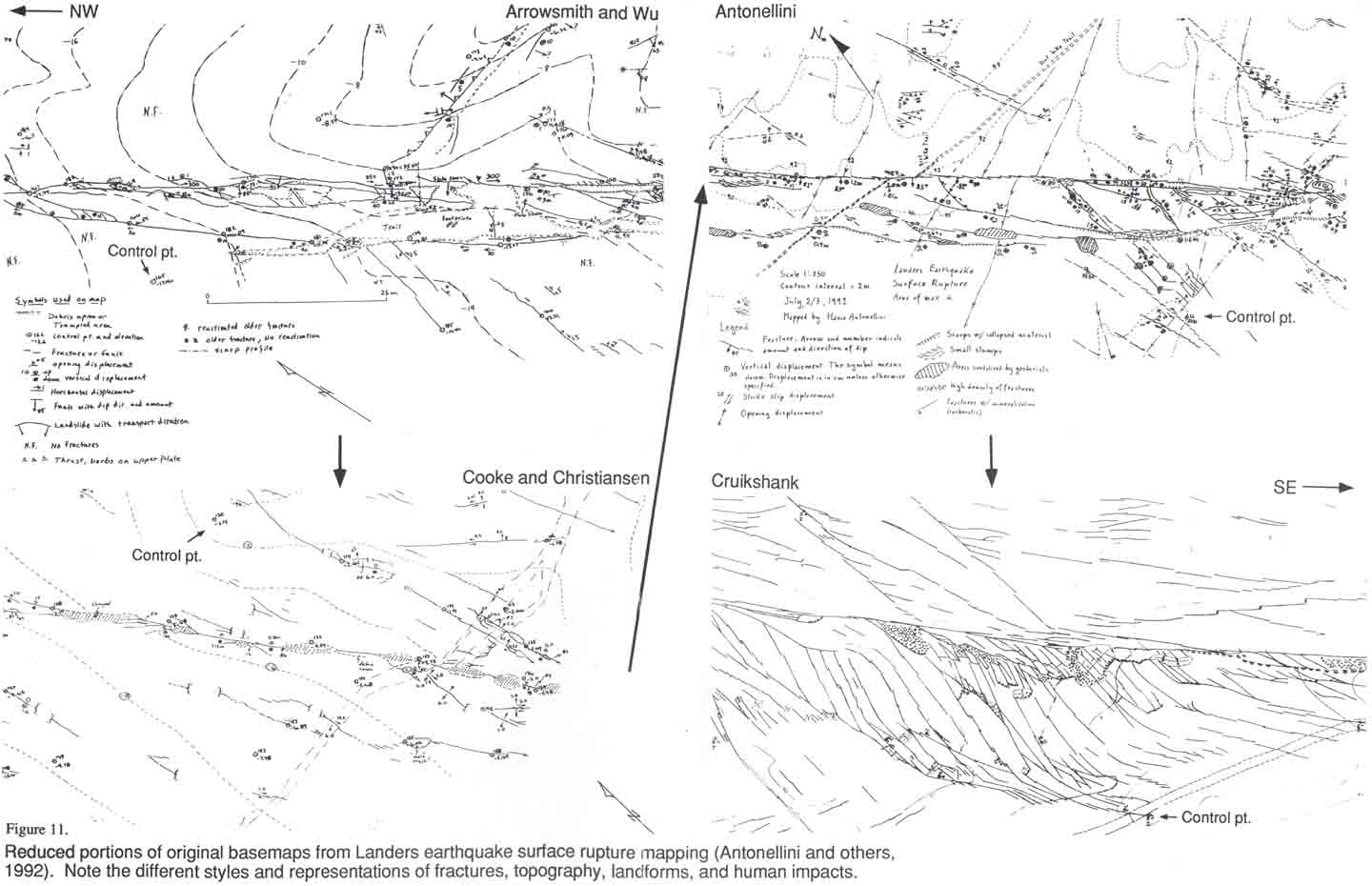
Figure 13. Final analytical fracture map from Landers study (compiled by Ken Cruikshank)..

Bibliography

Geologic mapping

Compton, R. R., 1985, Geology in the Field: New York, John Wiley and Sons, 398 p.

The best field geology book available. Covers all of the basics from rock identification through basic outcrop procedures to aerial photography. You should own it.

Electromagnetic distance measurement

Burnside, C. D., 1991, Electromagnetic distance measurement: Boston, Blackwell Scientific Publications, 278 p.

Good reference on the subject. A bit arcane in the explanation of the basics, but thorough. Includes a nice description of different equipment (3rd edition, TA601.B87 1991, Engineering Library).

Price, W. F., and Uren, J., 1989, Laser surveying: London, Van Nostrand Reinhold (International), 256 p.

Contains a good description of the basics of lasers, particularly GaAs diodes, and a clear description of the basics of EDMs. Covers other types of laser equipment as well (e.g., timed pulse distance measurement, alignment lasers, and laser Theodolites and levels), and laser safety (TA579.P94 1989, Engineering Library).

Basic Surveying

Moffitt, F. H., and Bouchard, H., 1987, Surveying: New York, Harper and Row, 876 p.

Good reference on the subject. This one has it all (8th edition, TA545.B7 1987, Engineering Library).

Advanced Surveying

Kennie, T. J. M., and Petrie, G., editors, 1990, Engineering surveying technology: New York, John Wiley and Sons (Halsted Press), 485 p.

Thorough overview of latest advances. Contains nice discussions of electronic distance and angle measurement, survey network errors, photogrammetry, and digital terrain modeling

Mapping reference

Antonellini, M., Arrowsmith, R., Aydin, A., Christiansen, P., Cooke, M., Cruikshank, K., Du, Y., and Wu, H., 1992, Complex surface rupture associated with the North Emerson Lake fault zone, caused by the 1992 Landers, CA earthquake: results of detailed mapping: EOS Transactions AGU, v. 73, p. 362.

---

Comments? e-mail Dr. Ramón Arrowsmith ramon.arrowsmith@asu.edu